Ideal Gas
 |
Contents |
The ideal gas model is used to help understand thermodynamics. The model is based on a few assumptions
- Large Number of Particles in the system
- The system follows the rules of Newtonian Mechanics
- Perfect Elastic Collisions
- Random Motion
Although the theory is based on assumption it describes systems with good accuracy. It isn’t perfect however and breaks down at low temperatures and high pressures, but so what, nobody’s perfect. Before we go any further it is worth going over some of the important equation for a gas.
If you put a gas in a box it will exert a pressure on the sides of the box. This is due to the gas particles hitting the sides with their random motion and providing a force. Force is defined as the rate of change of momentum so for 1 particle hitting the wall the force will be
![\[F=\frac{2mv}{\Delta t}\]](https://physicsforidiots.com/wp/wp-content/ql-cache/quicklatex.com-33e82eae6aaa94c2ca6bfd149ef5f9a5_l3.png "Rendered by QuickLaTeX.com")
for the time interval  . The reason for the factor of 2 is to take into account the change in momentum of the particle. In a perfectly elastic collision the particle will go from having momentum in one direction to having the same amount of momentum in the opposite direction.
To work out the force from all of the particles all we have to do is add up the forces from the individual particles. However not all of the particles in the box are going to hit the wall at once, so we need to work out the probability of a particle hitting the wall in the time interval . In order for a particle to hit the wall it would need to be within a length of  of the total length of the box,
  .
.
![\[Probability = \frac{1}{2}\frac{v\Delta t}{L}\]](https://physicsforidiots.com/wp/wp-content/ql-cache/quicklatex.com-345b93e0ca8b44dad80b49234ad1ee03_l3.png "Rendered by QuickLaTeX.com")
The factor of 1/2 comes from the fact that, taking into account only one dimension of motion i.e only one set of the box walls, then on average only half of the particle will be travelling in the direction of the wall we are interested in. We can now use this probability to sum up the forces from all of the particles like so
![\[F_{total}=\sum\frac{v\Delta t}{2L}\frac{2mv}{\Delta t}\]](https://physicsforidiots.com/wp/wp-content/ql-cache/quicklatex.com-38f3cd3c3f15f3b3de29c8376c02951e_l3.png "Rendered by QuickLaTeX.com")
This simplifies down nicely to
![\[F_{total}=\frac{m}{L}\sum v^2\]](https://physicsforidiots.com/wp/wp-content/ql-cache/quicklatex.com-009b8fa63fa5f606600c3fb891365cb3_l3.png "Rendered by QuickLaTeX.com")
Notice that the particles mass and the length of the box have been taken out of the summation. This is because is a constant and we are assuming that  is the same for all of the gas particles. So all we have to do is sum up the velocity squared for all of the particles.
Before we do that however we can make a quick change. We are more interested in pressure than force and we know the two are related by area so we can use the force equation to work out the pressure of the gas.
(1) 
Now to work out the sum of  . It isn’t too hard to do and just requires some logical thinking. If you add up the speed of a bunch of particle and divide by how many you have you will get an average value of the speed, so it makes sense that if you add up the ‘s and divide by the number of particles you will get an average value of . So the sum of the ‘s is just the average value times
  , the number of particles. However because the sample is in the real world there are 3 dimensions of motion to take into account, so we just divide by 3. Simple. So our value for the sum of can be written as
![\[\sum v^2=\frac{1}{3}N\left< v^2 \right>\]](https://physicsforidiots.com/wp/wp-content/ql-cache/quicklatex.com-499e89fc3f1fbb25472433d2bae3795c_l3.png "Rendered by QuickLaTeX.com")
The angled brackets or chevrons denote that the value inside them is an average value, and in this case is called the Mean Square Speed. We can now put this value back into equation 1 and replace the LA on the bottom for V, as a length times an area is a volume.
![\[P=\frac{Nm\left< v^2 \right>}{3V}\]](https://physicsforidiots.com/wp/wp-content/ql-cache/quicklatex.com-2bad76a8f9141c428d549805b5c2d451_l3.png "Rendered by QuickLaTeX.com")
It makes things a bit easier at this point if we take the volume term to the other side to go with the pressure term like so
(2) 
This now gives equation 2 a form in which it makes it easier to solve for  . To solve it we need to introduce possibly the most important equation when dealing with ideal gases, The Ideal Gas Law
(3) 
where
- P is the absolute pressure (pascals).
- V is volume (
 ).
). - T is the absolute temperature (kelvins).
- n is the number of moles of the gas.
- N is the number of molecules.
 is the Boltzmann constant,
  J K
J K .
.- R is the gas constant, 8.314 J molK.
The law works with any consistent set of units, provided that the temperature scale starts at absolute zero, and the appropriate gas constant is used.
The law comes from the combination of Boyle’s law, Charles’ law, Gay-Lussac’s law and Avogadro’s law. Which of the two forms of the equation you use depends on what you know. If you know how many moles of the gas you have then you use  , whereas if you know how many molecules you have you use
  .
.
You can see that equation 3 has a  term like the one in equation 2, so we can equate them and rearrange for
![\[\left< v^2 \right>=\frac{3kT}{m}=\frac{n3RT}{Nm}\]](https://physicsforidiots.com/wp/wp-content/ql-cache/quicklatex.com-44a47abfc4c96b02114cb623a1a86175_l3.png "Rendered by QuickLaTeX.com")
Now that we have a way of calculating , we can also work out the internal energy of the gas. Since the only energy in the system comes from the motion of the particle the internal energy will just be the sum of the kinetic energies.
![\[E_{KE}=\sum\frac{1}{2}mv^2=\frac{mN\left< v^2 \right>}{2}\]](https://physicsforidiots.com/wp/wp-content/ql-cache/quicklatex.com-8d74fa57f1d96a798053484d99438ba6_l3.png "Rendered by QuickLaTeX.com")
So subbing in out two expressions for the value of the mean square speed we get two equations to work out the energy of the gas
![\[E_{KE}=\frac{3}{2}NkT=\frac{3}{2}RT\]](https://physicsforidiots.com/wp/wp-content/ql-cache/quicklatex.com-7076cf4819a6c35bbeb80aa733ad0848_l3.png "Rendered by QuickLaTeX.com")
Now, although these derivations we have made assumptions and simplifications, but I can assure you these equations are in agreement with what is observed during experimentation.
Speed
Annoyingly, there are a few different measurements of particle speeds that are important in the study of gasses and other particle distributions.
Although I have kept using , a more useful value is the square root of this, and is called the Root Mean Square (RMS) Speed.
![\[V_{RMS}=\sqrt{\frac{3kT}{m}}=\sqrt{\frac{3RT}{M}}\]](https://physicsforidiots.com/wp/wp-content/ql-cache/quicklatex.com-5cc64e5df185177d4a2b96cde7fee20c_l3.png "Rendered by QuickLaTeX.com")
Another important value is the average speed, which is found by summing  for all of the particles
![\[\left< v \right>=\sqrt{\frac{8kT}{\pi m}}=\sqrt{\frac{8RkT}{\pi M}}\]](https://physicsforidiots.com/wp/wp-content/ql-cache/quicklatex.com-8058f84fedc858ebb245f3c6be0f831d_l3.png "Rendered by QuickLaTeX.com")
And there is the most probable speed vm (or sometimes vp)
![\[V_{mp}=\sqrt{\frac{2kT}{m}}=\sqrt{\frac{2RT}{M}}\]](https://physicsforidiots.com/wp/wp-content/ql-cache/quicklatex.com-8b0e574f1da60ee0af8ce14ebe6117a6_l3.png "Rendered by QuickLaTeX.com")
This last value is obtained by differentiating the distribution of speeds to find the maximum. The distribution of particle speeds in a gas is given by the Maxwell Distribution.
The Maxwell Distribution
The Maxwell Distribution was calculated in the 1850’s by James Clerk Maxwell (the same Maxwell who did the Maxwell Equations). The distribution of speeds in a sample follows is described by the follwing equation
![\[dN(v)=4\pi N\left(\frac{m}{2\pi kT}\right)^{\frac{3}{2}}v^2e^{\frac{-mv^2}{2kT}}dv\]](https://physicsforidiots.com/wp/wp-content/ql-cache/quicklatex.com-1df3c4d4415a94933a5aabd26b06625b_l3.png "Rendered by QuickLaTeX.com")
The shape of this distribution and the positions of the different speed values are shown below
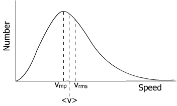
As you can see the graph crosses the (0,0) origin, this means that in a sample of gas there are no particles with a velocity of 0. A velocity of 0 would mean a temperature of 0 and an energy of 0, which would violate the uncertainty principle.
Transport Properties
Transport Properties are the properties of a material that relate to its ability to transport specific quantities, stuff like heat or mass. You can only get transport when the amount of ‘stuff’ varies from one place to another, if its the same all over then nothing is going to move. You need non-equilibrium for transport.
The 3 main transport properties that I will be attempting to explain are
- Diffusion – The Transport of Mass
- Viscosity – The Transport of Velocity
- Thermal Conductivity – The Transport of Energy
The transport properties are all related to how the particle in the material move and behave, so before we jump into the transport properties we will first need some more information, specifically information about Mean Free Paths and collision times.
Free Paths and Collisions
The average distance a particle travels between collisions is called The Mean Free Path. Assume you have a particle with a radius of  moving with a velocity ,
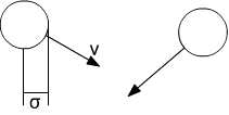
You can clearly see that you will only get a collision every time the distance between the centres of two particles is  . Knowing this we can simplify the situation to make things easier for ourselves. We will now assume that we have one particle of radius and all of the other particles are stationary points. This isn’t the case in real life, but it works for the calculations.

In a time interval the particle will move a distance of . If we look at the cross sectional area of our particle we see it will sweep out a volume of  . If there are
  stationary points in this volume then there will be
![\[nv\Delta t4\pi\sigma&2\]](https://physicsforidiots.com/wp/wp-content/ql-cache/quicklatex.com-0aef1d8bf63e3c97f86def4263350aa8_l3.png "Rendered by QuickLaTeX.com")
collisions per . To find the total we just do what we’ve been doing a lot of, sum over all of the particles, and we get a Collision Frequency,  , of
, of
![\[\gamma=2\pi\sigma^2n^2\left<v\right>\]](https://physicsforidiots.com/wp/wp-content/ql-cache/quicklatex.com-90c0ce2e231fb692e369bee738a24d18_l3.png "Rendered by QuickLaTeX.com")
collisions per unit time, per unit volume. We have divided by 2 as we are assuming each collision involves 2 particles, and the extra comes from the fact that we have summed all of the ‘s which is  .
.
If we wanted to find the distance between the collisions all we have to do is divide the distance the particle travels by the number of collisions it would have in that distance. This gives us a Mean Free Path,  , of
, of
![\[\lambda=\frac{v\Delta t}{nv\Delta t4\pi\sigma^2}=\frac{1}{4\pi n\sigma^2}\]](https://physicsforidiots.com/wp/wp-content/ql-cache/quicklatex.com-356c67233324a54f769ea0d47ad90a6b_l3.png "Rendered by QuickLaTeX.com")
It turns out that in getting to this formula one of our assumptions was slightly wrong. The calculation of the mean free path should take into account that all of the particles in the gas are moving. To do this we need to replace the speed of the particles with their relative speed as we are using the viewpoint that we are sitting on one particle moving and the rest are stationary. After many tedious calculations we find that all we have to do to make the equation accurate is add a factor of  . So the equation should be
(4) 
It is worth noting that this equation only holds for ideal Gases that follow the Maxwell distribution, so at low pressure or high temperature it will not hold.
Viscosity
Viscosity is a measure of a gas or liquids resistance to shear forces, forces parallel to a surface. Viscosity,  , is defined as
(5) 
but this isn’t a very nice formula so we will have to come up with a better one.
In order to calculate viscosity we will use the 6 streams method. The 6 streams refer to the positive and negative parts of the 3 axis of dimension. The speed a particle will have in the gas will depend on where they are, it will depend on their temperature which will vary from place to place.

Let’s assume that in the diagram above the particles have a fixed speed of  . The number of particles arriving at
  in a time will be
(6) 
This comes from the fact that in the time particles will travel a distance of , so only the particles in the volume  (the dotted voloume in the image) will be able to reach . is the number of particles per unit area and the 1/6 comes from the fact that only 1/6th of the particles in that volume will be moving down. The average velocity of the particles will be plus any change due to their velocity before. This can be expressed as
(7) 
is the mean free path length and ( ) is just the term that describes how the velocity varies with position. The change in momentum at will just be the momentum of the particles times the number of particles at . The number of particles at was calculated by equation 6 and the momentum can be obtained by multiplying equation 7 by , so we get
(8) ![\begin{equation*} \frac{dp}{dt}=\left[\frac{1}{6}An\left<v\right>\right]2\left[m\lambda\left(\frac{dv_{x}}{dy}\right)\right] \end{equation*}](https://physicsforidiots.com/wp/wp-content/ql-cache/quicklatex.com-732fa65c5d69ff7e15498196f7b7e48c_l3.png "Rendered by QuickLaTeX.com")
The 2 comes from the fact that particles can reach from above and below, and the term was taken to the other side to give dp/dt, the rate of change of momentum. The rate of change of momentum is force, so
![\[F=\frac{1}{3}Anm\left<v\right>\lambda\left(\frac{dv_{x}}{dy}\right)\]](https://physicsforidiots.com/wp/wp-content/ql-cache/quicklatex.com-372490739fccfc9ff4f7bde8a44231b0_l3.png "Rendered by QuickLaTeX.com")
Using the definition of viscosity given in equation 4, we can get the Equation of Viscosity as
(9) 
Which can also be written as
![\[\eta=\frac{m\left<v\right>}{12\pi \sigma^2}\]](https://physicsforidiots.com/wp/wp-content/ql-cache/quicklatex.com-d485ce71fc79be20531a54604b847cba_l3.png "Rendered by QuickLaTeX.com")
by substituting as given by equation 4. Unlike some of the other equations that only give close estimates, this equation gives an exact numerical value. From these equations you can see that Viscosity, , is independent of pressure
Thermal Conductivity
Thermal conductivity is the transport of heat energy and is represented as a greek kappa,  . is defined as
(10) 
Thermal Conductivity can be analysed the same way as we did for viscosity. The only difference being that we swap the momentum term for an energy term. So instead of equation 8 we get
(11) ![\begin{equation*} \frac{dE}{dt}=\left[\frac{1}{6}An\left<v\right>\right]2\left[\lambda\left(\frac{dE}{dy}\right)\right] \end{equation*}](https://physicsforidiots.com/wp/wp-content/ql-cache/quicklatex.com-0eb72ef8b636eaabeb7ba9bc866ca31b_l3.png "Rendered by QuickLaTeX.com")
where the momentum term of  has been replaced by the energy term
  . is the energy gradient of the gas, is tells you how the energy varies as you move around. This can be converted to a temperature gradient with a sneaky little maths trick like so
![\[\frac{dE}{dy}=\left(\frac{dE}{dT}\right)\left(\frac{dT}{dy}\right)\]](https://physicsforidiots.com/wp/wp-content/ql-cache/quicklatex.com-ec465d2e3ca2e05c77b16cf95006af96_l3.png "Rendered by QuickLaTeX.com")
Which we can sub straight back into equation 11 to get
![\[\frac{dE}{dt}=\frac{1}{3}An\left<v\right>\lambda\left(\frac{dE}{dT}\right)\left(\frac{dT}{dy}\right)\]](https://physicsforidiots.com/wp/wp-content/ql-cache/quicklatex.com-6c4da7470accb4743d08a0b2c6eac445_l3.png "Rendered by QuickLaTeX.com")
Combining this with our definition of thermal conductivity in equation 10 we get an Equation for Thermal Conductivity
(12) 
We know what equals from equation 4, so we know that is also independent of pressure, and also .
 is the heat capacity of the gas, it’s the ratio of how much heat energy you to transfer to an object compared to how much its temperature increases by. Heat capacity is usually referred to as
  , so we can slightly simplify our expression to
(13) 
Diffusion
For diffusion you really need 2 different gases, one gas on its own can’t really diffuse. However if you have 2 gases things can get complicated as they will have different masses and diameters. As we dont like things to be complicated (unless we’re doing quantum mechanics) we will just assume that the two gases have the same mass and same diameters. For things like air, or isotopes this works really well.
Diffusion, is defined by Ficks Law as
(14) 
Where j is the amount of stuff that will flow through a small area during a small time interval, D is the diffusion coefficient, the thing we want to work out, and (dn/dy) is the concentration gradient, it just tells you how the amount of stuff varies with position.
Like we did with thermal conduction, we will use the results of viscosity to help our working, only this time we will replace the momentum gradient with a concentration gradient. So we get
(15) 
Which we can just stick straight into equation 13 to get an Equation for Diffusion
(16) 
Relations
We now have 3 equations for the transport properties, describing Viscosity (η), Thermal Conductivity (κ) and Diffusion (D).
(17) 
(18) 
(19) 
As you can see these equations have some common features and can be combined to obtain relationships between η, κ and D. By combining the equations for D and η we get
(20) 
(21) 
where ρ is the density. And by combining the equations for κ and η we get
(22) 
((dE/dT) was replaced for Cv/Na) where Cv is the specific heat at constant volume, Na is Avogadro’s number and M is the molar weight.
Experimental values for equation 15 vary from 1.3 to 1.5 and values of equation 16 vary from 1.5 and 2.5. This is because real gases do not behave like ideal gases.
Now let’s see if we can apply this theory to electrons.
Classical Electrons
In 1900 the kinetic theory was applied to the problem of conduction in metals. It was assumed (by now you might be getting the impression that assuming things is all that scientists do) that in the absence of a magnetic field the electrons would move freely in the metal and because they had mass they would behave like an ideal gas and obey the kinetic theory. Lets see how far this assumption got them.
Density
How many electrons would you expect in a metal? The number of free electrons should relate to conductivity as we are assuming the electrons are doing the conducting. But conductivity has a huge range, spanning 25 orders of magnitude. This is the largest range for a physical parameter in the universe. The first estimate will be one free electron per atom. That seems ok doesn’t it? This gives about 1028-1029 electrons per m3 for metals.
Conductivity
If we are assuming the electrons are an ideal gas then the average velocity will be 0 (If it were anything else the sample would be moving across the room). If we apply an electric field to the sample then the electrons will be accelerated in the direction of the field. This will then give them a drift velocity. It is this drift velocity, vd that causes a current. If we have one electron in the field then it will follow Newtons law
(23) 
If the field is of strength E, then the force on the particle will be eE, and if we replace acceleration for the rate of change of velocity we get
(24) 
If we once again sum over all of the particles in the sample we get
(25) 
‹vd› is the average drift velocity in the direction of the field. According to this equation the velocity will increase with time, so a current should increase in a steady field. This isn’t what happens, however we can explain this because the electrons will collide with atoms, slowing them down and randomising their motion. So the electrons will only be accelerated for a time, τ. If we integrate equation 25 with respect to time we get the Electron Drift Velocity
(26) 
We also know the current density of the electrons, J. Its just the number of them, n, times their charge, e, times their velocity, ‹vd›,
(27) 
Combining equations 26 and 27 we get a relationship between current density and field
(28) 
Which is Ohms Law! Looks like we’re on the right track. We can use this then to get an expression for conductivity, σ (You will have to bear with me here. I know in the first section I introduced σ as radius but it is also used as conductivity. It could get a bit confusing, especially since they are going to appear in the same formula soon. I will try my best to make it clear which is which), as σ=J/E the Electrical Conductivity is
(29) 
Between collisions an electrons speed in increased by ‹vd›, so its kinetic energy in increased by 1/2m‹vd›2. This extra energy represents the heating of the wire the the current is going through. This heating is proportional to E2, a property that has been proved experimentally.
We have a correct law and a measured effect out of the theory. So far so good.
Now let’s try and get a value for τ. Electrons are very small, so they will only collide when they get within an atomic radius σ. Using the same working we did here we get an expression for the electron mean free path
(30) 
As you know, time is equal to distance over speed so τ is just
(31) 
I dont know why it is ‹1/vd› as opposed to 1/‹vd›, but it just is (probably something to do with some horribly complex maths). We can find the value of ‹1/vd› from the Maxwell distribution and it is
(32) 
So τ becomes
(33) 
So if we now combine equations 30 and 33 and put them into equation 29 we get an expression for Electrical Conductivity
(34) 
where the κ2 in the denominator is atomic radius. The fact that there is an e2 term show we are on the right lines. It shows that electrical conductivity is independent of charge sign i.e. Electrical Conductivity is always Positive. This equation also shows that the electrical conductivity, κ, is proportional to T -1/2
Thermal Conductivity
Good electrical conductors are the best thermal conductors. However thermal conductivity doesn’t have the same huge range as electrical conductivity. Thus free electrons cannot be responsible for all of the thermal conductivity of a metal. To work out the thermal conductivity κ for the electrons we will just use equation 13 that we came up with for an ideal gas with the temperature gradient replaced by the specific heat of electrons
(35) 
Substituting in equation 30 for the mean free path of electrons we get
(36) 
Values for the transport coefficients are only accurate to within a factor of 2, so we can forget the multiplying constants of the order 1, and we get
(37) 
This is our equation for the Thermal Conductivity of Electrons. Note that from equation 22, the τ term contains a T -1/2, which combines with the T in the numerator to give κ a T1/2 dependence.
Wiedemann-Franz Law
If we assume for the moment that all of the thermal conductivity in a metal is due to the electrons, then the ratio of conductivities would be simply
(38) 
Thus if all or most of the thermal conductivity was due to electrons then this ratio should be the same for all metals (at a set T).
Experimental Tests
We know, and have checked experimentally, that it is the electrons that are the things that cause the conduction. So that part of our theory is correct. What about the values of conductivities? Do the predicted values match with those found experimentally?
The Wiedemann-Franz Law (equation 38) predicts the ratio of conductivities as
(39) 
Experimentally it was found to be
(40) 
This is a satisfactory agreement; however it can be improved with a more detailed set of calculations, which keep a better track of constants than we did. But out rough theory definitely fits.
What about the temperature dependence of σ and κ? Experimentally the electrical resistivity, ρ, (inverse of conductivity) goes as
(41) 
At room temperatures ρ1(T) varies linearly with T, and at low temperatures ρ1(T) varies as T5. According to equation 23 σ∝T -1/2 so ρ∝T1/2, but this doesn’t match with experiment. Also, from equation 24 κ∝T1/2, however experimentally κ is found to be virtually independent of T.
And it was all going so well.
Specific Heat of Electrons
Using the Maxwell distribution you get that electrons have an average thermal energy of 3/2kT, this means they have a specific heat of 3/2nk per unit volume.
At room temperature the specific heats of metals and insulators are about the same and are independent of T. This suggests thatElectrons contribute very little to the Specific Heat of a Metal. This is only possible if the electron density is low.
So let’s lower the density, see what happens. If we lower it by about 0.01 so we get a density of about 1027 we get a relaxation time of about 10-12s. This gives us a speed for the electrons of about 105m/s, This may seem a bit big but remember that electrons are a lot lighter than your average gas particles. This speed gives us a mean free path of 10-7m. This is very large. We would expect them to only be able to get an atomic spacing before hitting something, usually an atom. All these numbers are consistent with An Electron Density higher than the Atomic Density. But we made a point of setting the density almost 100 times lower than the atomic density at the start.
Once again we have a problem.
But don’t worry, it isn’t all bad. The theory contains a lot of correct physics. The things responsible for the conduction are the free electrons, and we got Ohms Law and the Wiedemann-Franz Law out of it. It would be a huge coincidence if those laws had just fallen out of the theory randomly, so we’re at least partly correct. The problem comes from the specific heats and the temperature dependence of the conductivities. Both of which arise from the Maxwell Distribution. Maybe electrons don’t follow this distribution. Instead we will have to employ the deep dark magics of Quantum Mechanics to solve the problem.
Quantum Electrons
Our problem with the kinetic theory was that the Maxwell distribution didn’t apply to electrons. So we need to find a distribution that does. A good place to start would be to experimentally find out how the electrons behave, rather than just trying to come up with a theory blindly. One famous electron experiment is the photoelectric effect.
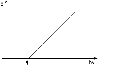
For the photoelectric effect you just shine a light on a metal and electrons are emitted. No one could explain why until Einstein came along in 1905, he said that the photons of light carry energy. The amount of energy they have is equal to their frequency times planks constant, and it is this energy that is transferred to the electron which can use it to escape the metal. Einstein came up with the following equation to explain this process.
![\[E_{Max}=hv-\phi\]](https://physicsforidiots.com/wp/wp-content/ql-cache/quicklatex.com-8aabf9db4875e581daebb10d955f889f_l3.png "Rendered by QuickLaTeX.com")
Where  is the maximum energy an electron can leave the metal with, and
  is the work function, basically the amount of energy it takes an electron to work its way out of the metal. This relationship can be shown graphically as
The electrons energy is measured with another metal plate above the one that is emitting the electrons. This second plate is charged so you can vary the charge so that only electrons with enough energy can get through. If you keep the frequency of the light constant and vary the charge on the second plate you get the following graph.

As all the electrons are getting the same amount of energy from the light then they must have started out in the metal with different amounts of energy, otherwise the graph would be a straight line. With a bit of maths and physics it was found that the distribution of the energies inside the metal was

So now all we have to do is come up with a theory and an equation that describes this distribution and we can solve the problems we had with the specific heat and conductivities.
The Sommerfeld Model
The model we want was developed by Arnold Sommerfeld, a German physicist who was one of the fathers of quantum mechanics. He decided that he was going to describe solids as big potential wells, with the potential inside the metal being 0 and it rising abruptly at the surface confining the electrons. He derived the potential by simplifying the sum of the potentials of all of the ions inside the solid. In reality it will be more complex than this having a periodic crystal structure, however for most solids this structure is very weak and can be ignored. This model now called the Sommerfeld Model after him is also sometimes referred to as the ‘Bathtub Model’. You can see why from the diagram below that represents the potential of the solid and the confined electrons.
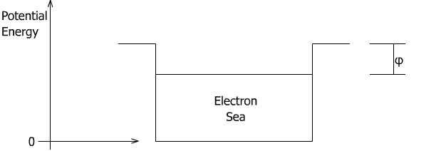
In the model Sommerfeld assumed that each atom contributes its valence electron i.e. Sodium atoms would give 1 electron, Aluminium atoms would give 7 etc. This assumption has since been experimentally verified. In order to make things easier the potential is assumed to be infinite square well (Unless we are considering the work function).
According to Quantum mechanics electrons have wave like properties and when confined to a potential well they can only occupy discrete states (For more info see here). By working out these states for a 3D infinite square well we can find the energy levels and hence the energy distribution.
Infinite Square Well
For an infinite square well the allowed energy levels are given by the following formula (The derivation of this formula can be found here).
(42) 
where L is the width of the well and n is the level number, with the lowest level being n=1. So from this we can work out the distribution of energies. First however I need to introduce one of the main rules of quantum mechanics, The Pauli Exclusion Principle. The Pauli Exclusion Principle stated that no two electrons can occupy the same quantum mechanical state, and this basically means you can never have 2 electrons in identical situations in a quantum state, something has to be different between them. For, when you are building an atom from scratch you start off with the nucleus and then add an electron, now if you want to add a second electron it has to have something different to the first. In this case it will be its spin. Electrons have a property called spin, which can be defined as being up or down, so the second electron you add to the atom will have the opposite spin to the first. Now what about if you want to add a third electron? There are only two possibilities for spin so something else will have to change, so the third electron creates the 2s shell to go into thus being in a different quantum state to the other two, and will more electrons the process continues, thus building up the periodic table. The exclusion principle also dictates how atoms and molecules interact and explains why matter doesn’t just fall through the massive gaps in atoms, it just isn’t allowed to. So with this one principle we have explained most of chemistry.
So the Pauli exclusion principle says that we can get 2 electrons on each of the energy levels, one of them spin up and one spin down. So to fill the potential well you just add the electrons one at a time, two to a level, starting from the lowest level (n=1) until you run out of the electrons that the atoms in the solid have supplied.
As we are dealing with a 3D well we need to convert equation 42 into a 3 dimensional equation which is just
(43) 
Degeneracy
It is worth making a quick note here about the situation known as degeneracy. Degeneracy is when you have two or more separate energy levels which have the same energy. For example if the value of were  ,
,  ,
,  , this would give the exact same answer for the energy as
  , ,
, ,  , even though they are 2 physically different levels.
Density of States
Our equation for the energy of the states in an infinite 3D well is given by equation 26. Our value for L in this equation will be of the order 1 meter as we are describing a sample of metal not an individual atom. If we put 1m into equation 26 then we get
(44) 
In the photoelectric effect experiment the electrons were being emitted with energies of the order 1eV. To get these energies the n values have to be huge in order to make up 19 orders of magnitude. We know that n changes by 1 from one level to the next, so the states must be packed in very closely on order to fit them all in.
To help with all these closely packed states we introduce a concept know as the Density of States, D(E), which is defined as the number of allowed states in a specific energy range. If we treat the  ,
,  and
and  values like vectors representing the distance from the lowest energy then we can use Pythagoras Theorem to combine them back into one resultant vector like so
(45) 
The number of states with energy  will just be the number of states inside the sphere of radius n.
![\[N=\frac{4}{3}\pi n^3\times \frac{1}{8}\times 2\]](https://physicsforidiots.com/wp/wp-content/ql-cache/quicklatex.com-d7d261bea45e0cc82dc0a232af331683_l3.png "Rendered by QuickLaTeX.com")
The first part of this formula works out the volume of a sphere of radius , the factor of  at the end comes from the fact that for each of the energy levels you get 2 electrons (spin up and spin down) and the factor of 1/8 comes from the fact that if the values represent the “distance” from the lowest energy point then the sphere of radius would look like this
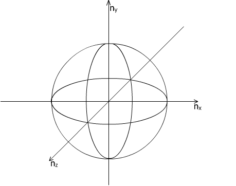
However, our values are only allowed to be positive, and only 1/8th of the sphere has all the values in it as positive, so that’s why we times by 1/8. If we do a quick bit of rearranging we get that is
![\[n=\left(\frac{3N}{\pi}\right)^{\frac{1]{3}}\]](https://physicsforidiots.com/wp/wp-content/ql-cache/quicklatex.com-46c577b6694e15c8b65a1fc0b8ae257d_l3.png "Rendered by QuickLaTeX.com")
which we can substitute back into equation 27 to get
![\[E_n=\frac{\hbar^2\pi^2}{2mL^2}\left(\frac{3N}{\pi}\right)^{\frac{2]{3}}\]](https://physicsforidiots.com/wp/wp-content/ql-cache/quicklatex.com-1802bf95322cb5be99a6a14751a720e4_l3.png "Rendered by QuickLaTeX.com")
We can also make the length term more useful. We know that  so
so  so
so  , which we can put in and then take inside the brackets along with the
  and get
(46) 
This is called the Fermi Energy,  and is the highest occupied state after all the available electrons have been piled in from the lowest states. Think of it as the surface of the electron sea in the bathtub model. From equation 28 you can see that most of the equation is made of constants and the energy only depends on the and
  terms, so we can write
![\[E\propto\left(\frac{N}{V}\right)^{\frac{2}{3}}\]](https://physicsforidiots.com/wp/wp-content/ql-cache/quicklatex.com-fdb92dd3875f1a8daf572a1686fa73de_l3.png "Rendered by QuickLaTeX.com")
But the number of electrons per volume is just the density, D, so we can write it as
![\[E\propto D^{\frac{2}{3}}\]](https://physicsforidiots.com/wp/wp-content/ql-cache/quicklatex.com-54924338cdc29c02e142705752f65dd9_l3.png "Rendered by QuickLaTeX.com")
Which we can rearrange for D to get
![\[D\propto E^{\frac{3}{2}}\]](https://physicsforidiots.com/wp/wp-content/ql-cache/quicklatex.com-7a0059a6a258c2b2ccd84ee07a350752_l3.png "Rendered by QuickLaTeX.com")
What we want to know however is how D varies with E, so we just differentiate with respect to E and get
![\[D(E)dE\propto E^{\frac{1}{2}}dE\]](https://physicsforidiots.com/wp/wp-content/ql-cache/quicklatex.com-a1883749fd24835f1ef9e32c6b125e0e_l3.png "Rendered by QuickLaTeX.com")
Which when plotted looks like this

Which bears a striking resemblance to the distribution we are looking for. The actual equation is given by
(47) 
Originally we assumed that each of the atoms gave one electron which gave us an electron density of about  –
– electrons per square meter. If we put this value into equation 28 we get
![\[E_f\approx10^{-18}J\approx 6eV\]](https://physicsforidiots.com/wp/wp-content/ql-cache/quicklatex.com-e99b333184256737b838c13af2829fbc_l3.png "Rendered by QuickLaTeX.com")
Which agrees with the results found in the photoelectric effect experiment.
The distribution we have just found and equation 28 and 29 apply when all the states are filled in order up to the Fermi energy, and this only applies at absolute 0 i.e. T=0K. But what about when T>0K?
Distribution at higher Temperature
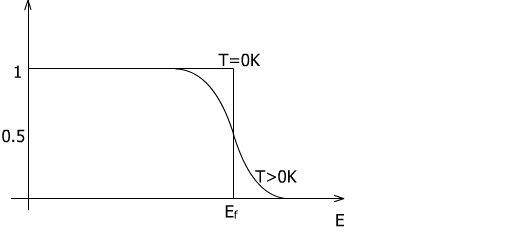
The distribution at higher temperatures depends on the probability of a state being occupied at a given temperature. This probability is given by the Fermi-Dirac distribution
(48) ![\begin{equation*} P(E)=\left[exp\left(\frac{E-E_f}{kT}\right)+1\right]^{-1} \end{equation*}](https://physicsforidiots.com/wp/wp-content/ql-cache/quicklatex.com-f055fffa613108f98e4e746549f905f4_l3.png "Rendered by QuickLaTeX.com")
For  the probability is close to 1, you are very likely to find electrons below the Fermi energy at most temps. For
  the probability is almost zero. At
  is is exactly a half as you can see from the equation. Because of the exponential term, P(E) is usually 1 or 0 except for a small region around the fermi energy. The following graph shows the probability at T=0 (sharp cut-off at ) and at some value of T higher than 0 (slope across )
So now if we include this probability into our equation then our distribution is given by
![\[P(E)D(E).dE\]](https://physicsforidiots.com/wp/wp-content/ql-cache/quicklatex.com-7a720bbd6dc5c4f57d50433b4df6ea3a_l3.png "Rendered by QuickLaTeX.com")
Which will give us the following graphs

which is the distribution we were looking for! So now we have a working theory and set of equations that describe the distribution of electrons and their energies.
Before we move on let’s just look in more detail at the situation where  . Our P(E)D(E) equation becomes
![\[P(E)D(E)dE\approx exp\left(-\frac{E-E_f}{kT}\right)\times AE^{\frac{1}{2}}.dE\]](https://physicsforidiots.com/wp/wp-content/ql-cache/quicklatex.com-7d4ecd118175eb0d74e4527c86e27812_l3.png "Rendered by QuickLaTeX.com")
The first term is equation 30 and the second term is equation 29. The +1 from equation 30 has been missed out as the exponential will be large, and the fact that is should be 1 over the exponential is taken into account by making the exponential negative ( ). The constants from equation 29 have been combined into one constant, A, for the sake of simplicity. As then
  will just be
  , so we can rewrite the equation as
![\[P(E)D(E)dE\approx exp\left(-\frac{E}{kT}\right)\times AE^{\frac{1}{2}}\]](https://physicsforidiots.com/wp/wp-content/ql-cache/quicklatex.com-359483e5775a6339c97883f99dd14a0e_l3.png "Rendered by QuickLaTeX.com")
We also can replace E with the equation for kinetic energy
![\[E=\frac{1}{2}mv^2\]](https://physicsforidiots.com/wp/wp-content/ql-cache/quicklatex.com-45583fe3ad0e7bada20f0a475735919d_l3.png "Rendered by QuickLaTeX.com")
to get
![\[P(E)D(E)dE\approx Bv^2exp\left(-\frac{mv^2}{2kT}\right)\]](https://physicsforidiots.com/wp/wp-content/ql-cache/quicklatex.com-57a42c2d26bc09701b92dd0007bb8e58_l3.png "Rendered by QuickLaTeX.com")
Which is the Maxwell Distribution!!! Now let’s see if we can use this new distribution to take care of the problems we got the first time round
Specific Heat of Electrons 2
The energy distribution of electrons changes depending on temperature
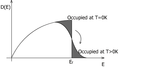
The electrons can only be excited to higher states if there is a free state for them to go in to. Thermal excitations are usually a few kT’s in energy so only the electrons which are a few kT’s from the fermi energy can be excited (The rest are trapped in below without enough energy to be excited up through multiple levels).
The number of electrons that can be excited is equal to the shaded area. This area is roughly equal to the density of electrons at the fermi energy times the width kT, so D(Ef)kT. The total number of electrons is roughly given by the density at the fermi energy times the width Ef (It’s a rectangle of width Ef and height D(Ef), which is a very rough estimate). This means that the ratio of electrons excited is
![\[\frac{D(E_f)kT}{D(E_f)E_f}=\frac{kT}{E_f}\]](https://physicsforidiots.com/wp/wp-content/ql-cache/quicklatex.com-abec1e6c6e20d3307560b202a968530b_l3.png "Rendered by QuickLaTeX.com")
So the total number of electrons excited will just be this fraction times the number of electrons N. Specific heat is the measure of energy it takes to increase the heat, so the energy increase will just be the number of electrons excited times by the energy of excitation, which is kT, and then to get the specific heat we just divide by temperature (So we get energy/temp, or energy per unit temp). This gives
![\[C_v=\frac{Nk^2T}{E_f}\]](https://physicsforidiots.com/wp/wp-content/ql-cache/quicklatex.com-d870aea523e78c99255acc88d72bd47f_l3.png "Rendered by QuickLaTeX.com")
The classical value of the specific heat was about Nk so the difference is kT/Ef. This difference is usually of the order 0.01 or less which means that the electrons contribute very little to the specific heat of the metal, mainly because most of them are trapped in the lower levels. The equation we obtained for the specific heat uses some very rough estimations. If you use more detailed calculations you get
(49) 
which shows that even our rough estimation were pretty correct (only out by a factor of 5).
Conductivity 2
Just like before we are using the idea that conductivity arises from the electrons gaining a drift velocity from an eternal field, however this time we have to take into account the pauli exclusion principle. The main difference between the classical and quantum descriptions comes from the mean free path. For an electron to scatter it must have a free state to scatter into, so only the electrons around the fermi energy can do this. Their velocity will correspond to the the fermi energy so we have
![\[\lambda=v_f\tau\]](https://physicsforidiots.com/wp/wp-content/ql-cache/quicklatex.com-6d83b5daee2d983dc3d36b2aa9fe7226_l3.png "Rendered by QuickLaTeX.com")
The equation for conductivity is the same as before (equation 20)
![\[\sigma=\frac{ne^2}{m}\tau\]](https://physicsforidiots.com/wp/wp-content/ql-cache/quicklatex.com-4cf2a1164480272293a5872f60d7db18_l3.png "Rendered by QuickLaTeX.com")
Which when combined with the new mean free path gives
(50) 
The fermi velocity is independent of temperature and varies with T, so  which means that resistivity is proportional to
  , which was found here.
Thermal Conductivity 2
We will use the 6 streams method as we did before so we get the thermal conductivity as
![\[\kappa=\frac{1}{3}\left<v\right>\lambda\frac{C_v}{N}\]](https://physicsforidiots.com/wp/wp-content/ql-cache/quicklatex.com-dfd23c8256068bbbd8a51a83085f13df_l3.png "Rendered by QuickLaTeX.com")
As we just stated, only electrons with at the fermi energy will be able to move around so we can replace the average velocity,  , with the fermi velocity
  . We can also replace the specific heat with the new one calculated in equation 31 to get
![\[\kappa=\frac{1}{3}nv_f\lambda\frac{\pi^2k^2T}{2E_f}\]](https://physicsforidiots.com/wp/wp-content/ql-cache/quicklatex.com-d89d5b77ea4161a46117e10c1b6c654b_l3.png "Rendered by QuickLaTeX.com")
We know that at high temperatures  , so is independent of , which is now correct. And at low temperatures is virtually independent of temperature so
  , which is again correct.
Wiedemann-Franz Law 2
Now that we have 2 new values for and we can now get a new value for the Wiedemann-Franz law, which is
![\[\frac{\kappa}{\sigma}=\frac{\pi^2}{3}\frac{k^2}{e^2}T\]](https://physicsforidiots.com/wp/wp-content/ql-cache/quicklatex.com-3fccf0b5d9df8bee9e751e8edfedbccc_l3.png "Rendered by QuickLaTeX.com")
which comes out as about  . This number matches the one found experimentally a lot better than before.
Pauli Paramagnetism
As well as electric fields the electrons inside a metal will also react to an applied magnetic field. Electrons have a magnetic moment due to their spin (Remember that a magnetic field is created by a moving charge, which includes a spinning electron). The magnetic moment of an electron,  , is given by
![\[\mu=-2\mu_{B}S\]](https://physicsforidiots.com/wp/wp-content/ql-cache/quicklatex.com-4f27f4dd1b50ec5cbce96be443e8b76f_l3.png "Rendered by QuickLaTeX.com")
where  is the spin vector and
  is the Bohr Magneton, which is equal to
![\[\mu_B=\frac{e\hbar}{2m}\]](https://physicsforidiots.com/wp/wp-content/ql-cache/quicklatex.com-883b5a09453afd2a76ba50717696ec9a_l3.png "Rendered by QuickLaTeX.com")
In a magnetic field the electrons will gain an extra  of magnetic energy depending on the direction of their spin, which will separate the up and down electrons. can be either ±1/2 for spin up or spin down so the extra energy that the electrons get will be either
  . Half the electrons will be spin up and half will be spin down ((1) In the diagram below), so half will get an increase in energy and half will get a decrease ((2) in the diagram below).
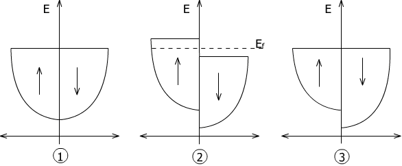
The electrons that gained energy will want to return to the lowest energy state, the fermi energy. To do this they will undergo a process known as spin flipping. This causes a net magnetic moment in the metal as there are now more electrons of one spin than the other. The net magnetic moment caused by the imbalance of electrons is equal to
![\[D(E_f)\mu_B^2B\]](https://physicsforidiots.com/wp/wp-content/ql-cache/quicklatex.com-0b5e8706350ea592d84039889d80dd22_l3.png "Rendered by QuickLaTeX.com")
The magnetization of a metal can be defined as the magnetic moment per unit volume, and the magnetic susceptibility can be defined as M/B, so we have
![\[M=\frac{\mu_B^2D(E_f)B}{V}\]](https://physicsforidiots.com/wp/wp-content/ql-cache/quicklatex.com-8becd3fd3a241b1f8e55be748906ed85_l3.png "Rendered by QuickLaTeX.com")
![\[\chi=\frac{\mu_B^2D(E_f)}{V}\]](https://physicsforidiots.com/wp/wp-content/ql-cache/quicklatex.com-9d97ca44d7fa9534ec536db6cbaceae9_l3.png "Rendered by QuickLaTeX.com")
Using the distribution at the fermi energy we can rewrite the susceptibility as
![\[\chi=\frac{3n\mu_B^2\mu_0}{2E_f}\]](https://physicsforidiots.com/wp/wp-content/ql-cache/quicklatex.com-896bcb45d03e0d9f721a6eff2ea9b862_l3.png "Rendered by QuickLaTeX.com")
The value of  is roughly
  and is in good agreement with experimental results.
The Hall Effect
What happens if you have an electric field and a magnetic field? To test this we take a thin rectangular slap of metal and apply a voltage across it and a magnetic field through it like so
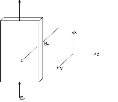
So we have an E field in the x direction and a B field in the y direction. To work out what happens we have to use the Lorentz Force Law
![\[F=e(E+v\times B)\]](https://physicsforidiots.com/wp/wp-content/ql-cache/quicklatex.com-108bf9dc3ccafd4fb2de495ae3758810_l3.png "Rendered by QuickLaTeX.com")
Due to the cross product between the velocity of the electron and the magnetic field the electrons move in a circular path like so
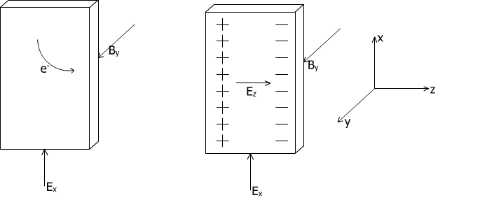
This creates an imbalance of charge in the metal that creates a third field, an E field in the z direction. When the system gets to equilibrium this E field cancels the effect of the B field and a normal current can flow. So if we solve the Lorentz equation we get
![\[F=e(E_z+v_xB_y)=0\]](https://physicsforidiots.com/wp/wp-content/ql-cache/quicklatex.com-3cc03bd8d86ed2c7a7272abf80af6baf_l3.png "Rendered by QuickLaTeX.com")
so
![\[v_x=\frac{E_z}{B_y}\]](https://physicsforidiots.com/wp/wp-content/ql-cache/quicklatex.com-406a87a9610896017e50c6b1e698dab8_l3.png "Rendered by QuickLaTeX.com")
The normal current that flows can be described by
![\[J=-env\]](https://physicsforidiots.com/wp/wp-content/ql-cache/quicklatex.com-436543e879f0c314ad6d39a0754eaa1f_l3.png "Rendered by QuickLaTeX.com")
Where is the electron density. If we substitute in the equation for the velocity that we got from the Lorentz equation then we get
![\[\frac{E_z}{JB_y}=\frac{1}{ne}=R_H\]](https://physicsforidiots.com/wp/wp-content/ql-cache/quicklatex.com-e15be5820191eb9cf45a097a90e1b89d_l3.png "Rendered by QuickLaTeX.com")
where  is the Hall resistance (as it has the units of ohms). As ,
  and
and  can be measured easily we can obtain direct measurements of the electron density.